My astronomy research focused on studying massive stars across the HR Diagram from hot OB and Wolf-Rayet stars, to cool yellow and red supergiants. During my years working at Lowell Observatory, as a PhD student at the University of Washington, and later as a postdoc, I regularly observed on telescopes in Chile, Hawaii, and Arizona to better constrain the numbers and types of massive stars in the Local Group galaxies M31, M33, and the Magellanic Clouds. My postdoctoral research focused on using these massive stars in binary systems to determine how they might someday merge to form gravitational wave events detectable by the Laser Interferometer Gravitational-wave Observatory (LIGO).
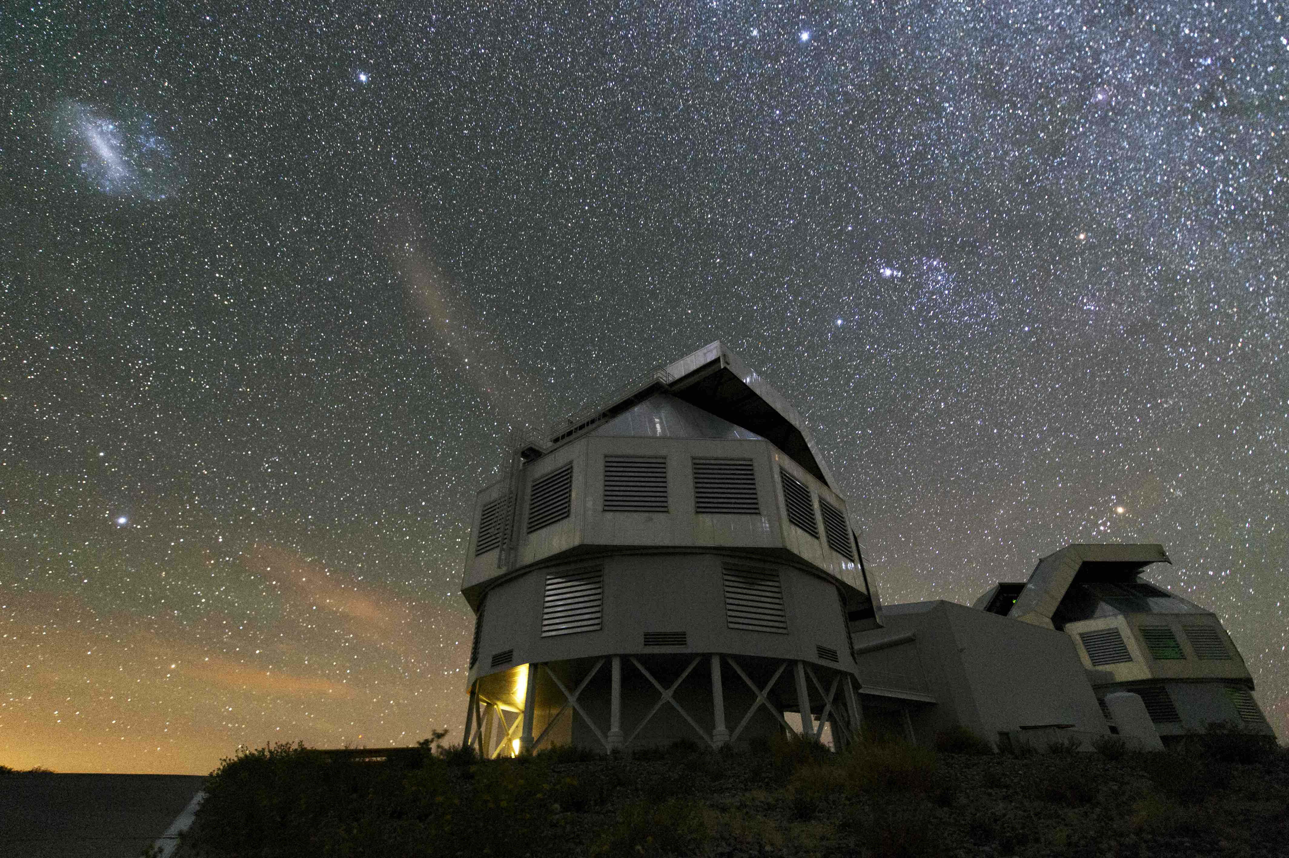
The amazing Magellan telescopes and the Large Magellanic Cloud.
Here I give a very brief overview of massive star astronomy and attempt to place my research into the greater context of why studying these objects is so exciting and important.
Why Study Massive Stars?
(because they’re awesome)
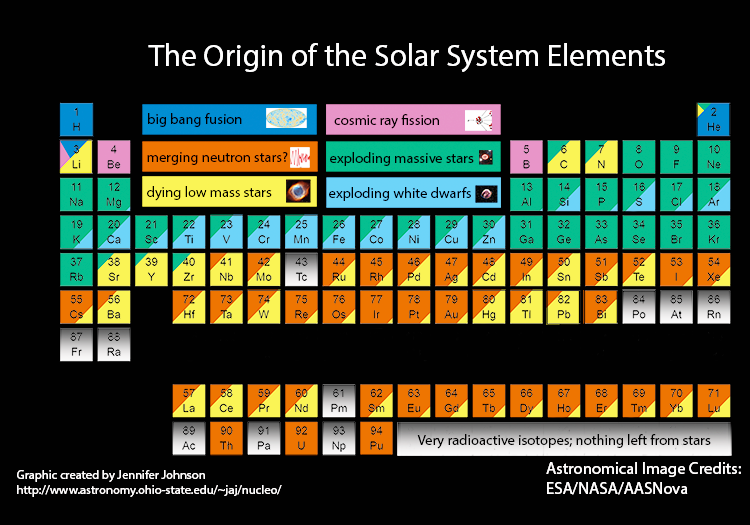
Massive stars are the cosmic engines of the Universe. The majority of the oxygen we breathe, the silver and gold we prize, and the carbon that allows for life as we know it, is created during the explosive death of a massive star. Furthermore, once these massive stars explode, they leave behind compact objects (like neutron stars) that may someday merge and create even more heavy elements. As the periodic table below shows, massive stars play a key role in creating the majority of the elements here in our Solar System.
Unevolved OB stars
How can we determine their physical properties?
Massive stars begin their lives as hot, hydrogen-burning OB stars that are greater than around 8 times the mass of our own Sun. I began my massive star research studying these OB stars at Lowell Observatory working with Dr. Phil Massey. I spent the summer of 2009 using the spectra of OB stars to determine their physical properties (such as temperature, luminosity, mass, and chemical abundances). I placed constraints on these properties by modeling the spectra with two different computer programs and then compared the results – one program made a lot of approximations but was quite quick to run, while the other solved the physics in much more detail but took a couple days for a model to converge. While these two programs are widely used in the astronomy community, a direct comparison between the results had never been done. In the end, we found that modeling the OB stars could be done quite reliably (with some caveats) using either program!
Yellow Supergiants
How long do they live?
After massive OB stars burn through their hydrogen, their evolutionary path is mass-dependent. Stars that are between 8 - 10 times the mass of our Sun evolve off the main-sequence and briefly pass through a yellow supergiant (YSG) phase that lasts only a couple hundred thousand years. Due to the brevity of this phase, coupled with the overall scarcity of massive stars, correctly predicting the lifetimes and thus populations of YSGs has long proved challenging for theorists. Initial studies found a factor of 10 discrepancy between the theoretical predictions for the lifetimes of these stars and observational data. But, it wasn’t clear whether the fault lay with the models or a lack of completeness in the observations.
My collaborators and I set out to identify a complete sample of YSGs in the Large and Small Magellanic Clouds (LMC, SMC). Before the Gaia spacecraft launched, the only reliable way to separate extragalactic YSGs from foreground Galactic yellow dwarfs was to obtain spectra. Using the CTIO 4m, we observed around 2500 stars in the SMC and LMC and used radial velocities to identify 800 YSGs. Our initial YSG luminosity function in the SMC showed that the evolutionary models predicted far more high luminosity YSGs than existed (see the figure below, left) and this discrepancy spanned across all metallicity regimes. After collaborating with our theoretician colleagues, improvements were made to how mass-loss and convection were treated in the evolutionary models. We then compared the updated models with our observational results in the LMC, and the agreement was excellent, as is shown in the Figure below on the right. As a result of my observations and collaborations, the evolutionary models are now able to reproduce the observed YSG luminosity distribution.
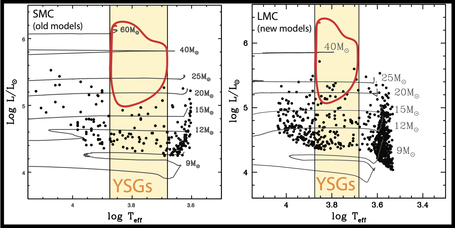
HR Diagrams of observed YSG populations with Geneva evolutionary tracks. Our initial study in the SMC (left) showed a lack of observed high luminosity YSGs that were predicted by the models. After improvements were made to the models, the agreement was much improved (right).
Wolf-Rayet stars
How Does Metallicity Affect Wolf-Rayet Populations?
The most massive stars (with initial masses greater than 30 times the mass of the Sun) don’t pass through the YSG phase but instead evolve directly into Wolf-Rayets (WRs). The evolution of these stars can be likened to peeling an onion layer by layer, with strong stellar winds doing the work. First, the hydrogen-burning products nitrogen and helium will be revealed, producing a WN-type WR. Next, if the stellar winds are strong enough, the helium burning products carbon and oxygen will appear, and a WC-type WR results. The strength of these stellar winds is based on the metallicity of the environment so it follows that more WC-type WRs will be found in areas of higher metallicity. Thus, comparing the number of WC to WN type WRs as a function of metallicity is an exacting test of stellar evolutionary theory. When I began my WR research, the models did a poor job of predicting the WC to WN ratio (see the figure below, left), but, like with the YSG population, we were unsure whether the fault was with the models or observations. Thus, we began a campaign to identify complete samples of WRs in the Local Group galaxies M31, M33, and the Magellanic Clouds.
To search for WRs, we imaged the entire optical disks of these galaxies with interference filters centered on the WR’s broad, strong emission lines. Using image subtraction of the interference images, paired with spectroscopic follow-up on Las Campanas in Chile and the MMT in Arizona, we found 54 new WRs in M33 bringing the total up to 206, 107 new WRs in M31 (total = 154), 16 new WRs in the LMC (total = 152), and confirmed that there are only 12 WRs in the SMC. As a result, the observed WC to WN ratio is now in agreement with both single star, and the newer binary star model predictions (see the figure below, right). Unlike with the YSGs, the disagreement between the WR models and observations was due to a lack of completeness in the observations, which was remedied through my discoveries.
However, it wasn’t just the number of new WRs that we found that was so exciting, but also their types. Ten of the new LMC discoveries are an entirely new class of WRs, which we’ve called WN3/O3s. These WRs show both strong emission similar to that of an early-type WN3 but also strong absorption like that of an O3V. However, due to their faint magnitudes, we know they are not WN3 + O3V binary systems. My Master’s thesis work at the Northern Arizona University focused on modeling these stars with the non-LTE spectral modeling program CMFGEN to determine a single set of physical parameters that reproduced the spectrum of each of these stars. I found that while their temperatures and luminosities are consistent with other LMC WNs, their mass-loss rates are much lower. The evolutionary status of these stars is still being debated within the massive star community: are they just a normal, short-lived evolutionary phase as O stars turn into WRs? Or have they been stripped by compact companions and will soon merge to create gravitational wave events?
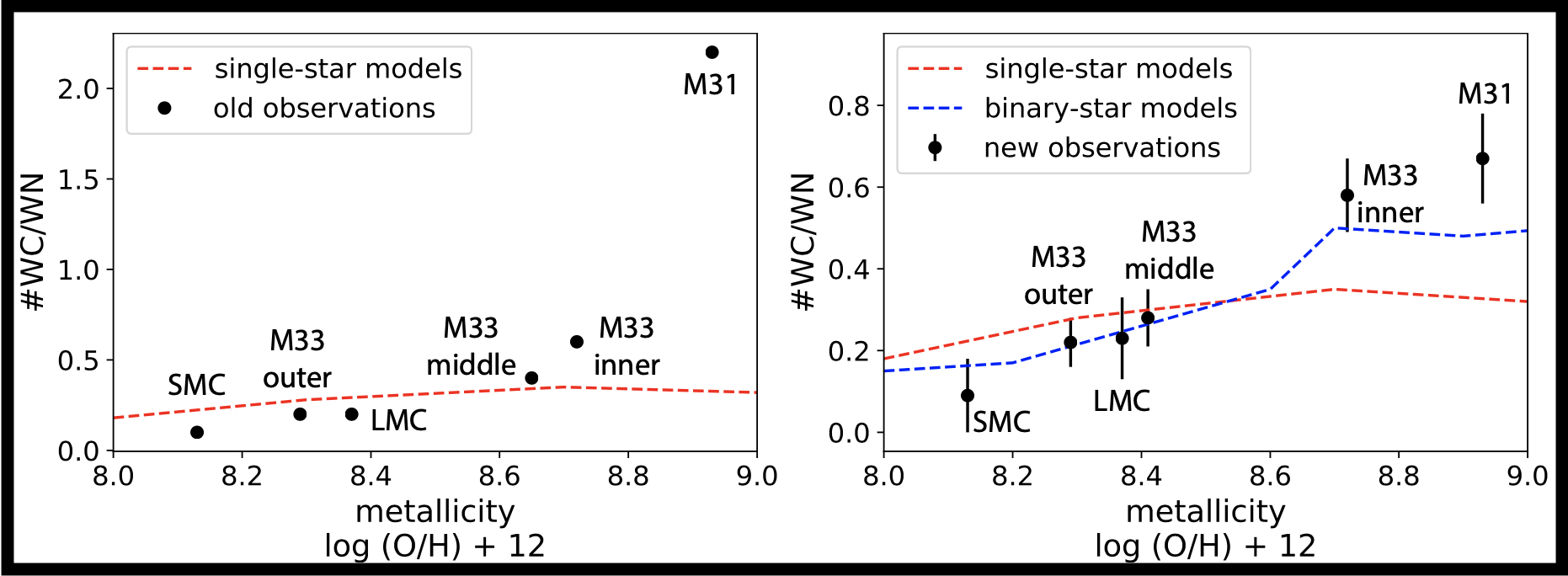
WC/WN ratio vs. metallicity. Note the vast improvement in the agreement between the observations and model predictions before I began this study (left) compared to when I finished (right). This was solved by my discovery of 177 new WRs in M31, M33, and the LMC.
Red Supergiants
What is the Binary Fraction of Red Supergiants?
For my PhD dissertation at the University of Washington working with Dr. Emily Levesque, I turned my attention to the coolest of the massive stars, the red supergiants (RSGs), and determined their binary fraction for the first time. The percentage of massive main sequence OB stars in binary systems is thought to be as high as 100%; however, when I began my research back in 2018, only around a dozen of their evolved descendants, the RSGs, were known to be in binary systems. I first studied the evolution of such systems and found that binary RSGs will primarily have B-type companions. Such systems will have unique photometric signatures due to the shape of their spectral energy distributions (see the figure below, left). I then went searching for these systems photometrically with spectroscopic follow-up using the 6.5m MMT and Magellan telescopes. In total, I found over 250 of them in the Local Group galaxies of M31, M33 and the Magellanic Clouds – increasing the known population by 20 times!
To identify the overall binary fraction of RSGs in the LMC, M31, and M33, we identified a complete sample of RSGs down to a log luminosity > 4.2 using Gaia to remove foreground stars and near-IR photometry to separate out the RSGs from bright asymptotic giant branch stars. After characterizing the range of color space where I expected RSG binaries to reside, I was able to estimate the overall binary fraction of RSGs as a function of metallicity across all three galaxies and found that there was a surprising decreasing trend with decreasing metallicity (see the figure below, right). This environmental dependence on the massive star binary fraction is not echoed in the evolutionary models and thus presents an interesting question for massive star evolution, including the creation of gravitational waves.
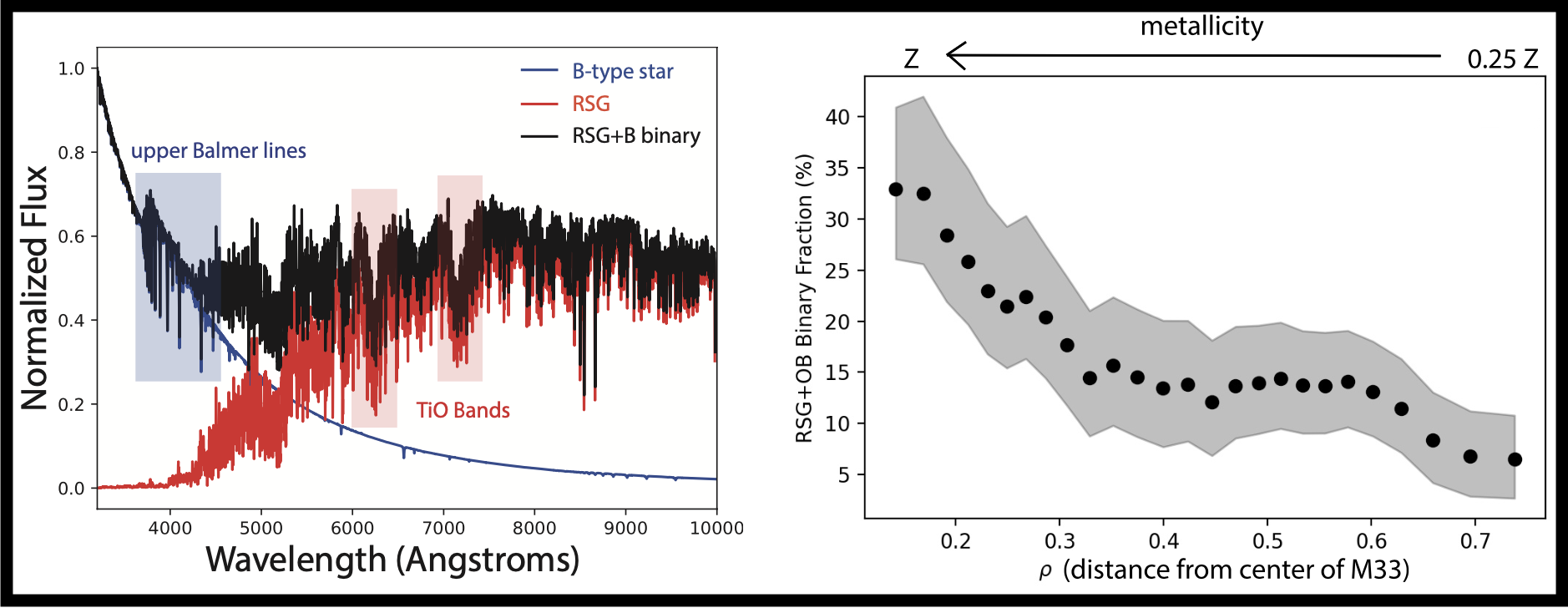
(left) Combined RSG+B star spectrum showing both the B star’s upper Balmer lines and RSG’s TiO bands. (right) M33 RSG+OB binary fraction as a function of decreasing metallicity.
Luminous Blue Variables
My feelings about LBVs can be summarized by this video.
What about non-massive star research?
Sky Brightness at Kitt Peak National Observatory
While working with Phil Massey at Lowell observatory, we measured the night sky brightness of Kitt Peak National Observatory near Tucson, AZ. We then compared our 2010 data to measurements taken by Phil in 1990 and 2000. Remarkably, we found that the brightness of the Kitt Peak night sky at zenith is just as dark as it was 20 years ago. This suggests that the lighting ordinances established in Tucson and Pima County in the early 2000s have been incredibly effective. Our efforts were highlighted by the Tucson newspaper as well as numerous other sources such as Sky & Telescope and a press release by NOAO.
Azimuthal brightness variations in Saturn’s rings
During my junior and senior years at Wellesley College I worked with Professor Richard French analyzing Saturn Cassini data. I spent the first semester investigating the azimuthal asymmetries in Saturn’s A and B rings using VIMS data. These asymmetries are caused by ring particle formations called wakes. Wakes are created by the inherent desire of particles to bind together through gravitational forces. However, these particles are within the Roche limit, meaning they can’t bond together and form a moon because of tidal disruptions from Saturn’s gravitational pull. However, the tidal disruptions do cause them to form small streams called wakes. These streams are tilted 20 degrees with respect to Saturn’s ring plane. Thus, depending on the tilt of Saturn’s rings and your viewing angle, it is either easier to see through the rings and the rings appear darker (trailing quadrant) or it is harder to see through the rings and thus the rings reflect more light back to you and appear lighter (leading quadrant). I then spent the second semester looking at ring occultation data and measuring the location of different prominent ring features (such as the Cassini and Encke divisions). This data can then be used to help determine the precise pole solution for Saturn.
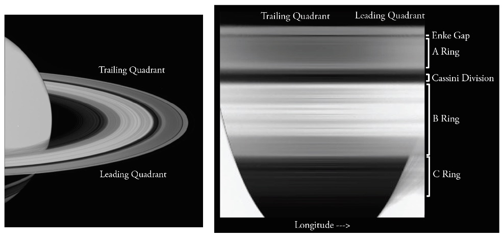
Notice the brightening (in the leading quadrant) and darkening (in the trailing quadrant). (French et al., 2007)
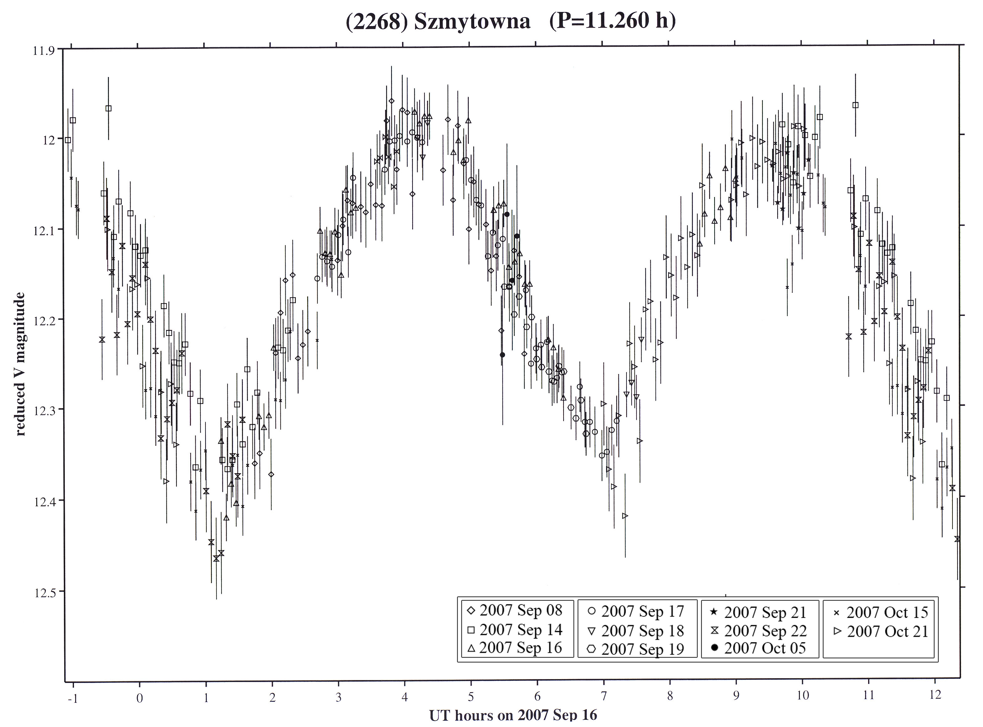
Koronis Family Asteroids
As a sophomore at Wellesley College I participated in the Sophomore Early Research Program. This research paired me with astronomy Professor Steve Slivan and his work on Koronis Family asteroids. During my first year of astronomy research, I learned how to use the 24-inch telescope at Wellesley’s Whitin Observatory to collect and reduce CCD images. I then used these images to determine the periods and H magnitudes for three different Koronis Family members: (3032) Evans, (1443) Ruppina, and (2268) Szmytowna. The light curve for (2268) Szmytowna phased to the appropriate period is shown below. At the end of the year, Professor Slivan and I published a paper in the Minor Planet Bulletin detailing our findings.